The Soil Composite Mapping Processor (SCMaP) is a new approach designed to make use of per-pixel compositing to overcome the issue of limited soil exposure due to vegetation. Three primary product levels are generated that will allow for a long term assessment and distribution of soils that include the distribution of exposed soils, a statistical information related to soil use and intensity and the generation of exposed soil reflectance image composites. The resulting composite maps provide useful value-added information on soils with the exposed soil reflectance composites showing high spatial coverage that correlate well with existing soil maps and the underlying geological structural regions.

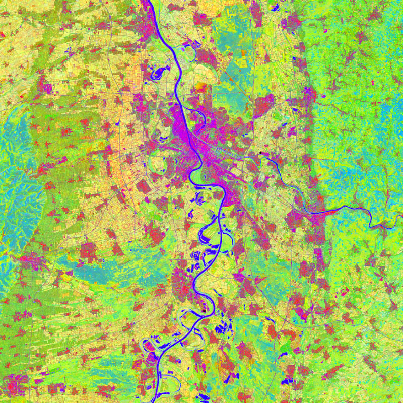
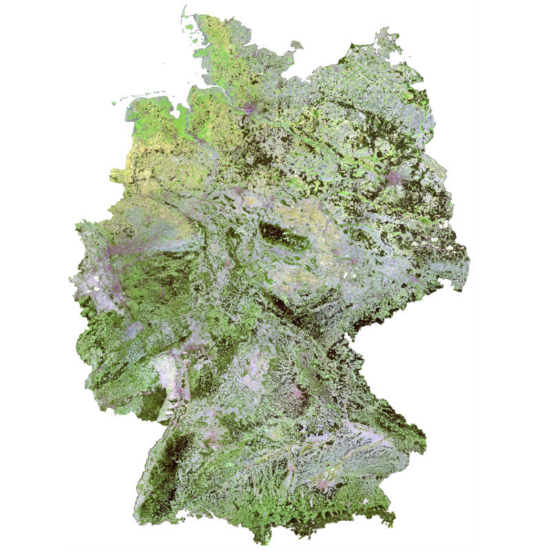
The TimeScan product is based on the fully-automated analysis of comprehensive time-series acquisitions of Landsat data. Based on a user-specified definition of the required period of time, the region of interest and – optionally – the maximum cloud cover, the TimeScan processor starts with the collection of all available Landsat scenes that meet the user specification. Next, for each single scene masking of clouds, haze and shadow is conducted using the Fmask algorithm. Then, a total of 6 indices is calculated for those pixels of each single scene that have not been masked in the prior step. The set of indices includes the Normalized Difference Vegetation Index (NDVI), the Built-up Index (BI), the Modified Normalized Difference Water Index (MNDWI), the Normalized Difference Band-5 / Band-7 (ND57), the Normalized Difference Band-4 / Band-3 (ND43), and the Normalized Difference Band-3 / Band-2 (ND32). Finally, the TimeScan product is generated by calculating the temporal statistics (minimum, maximum, mean, standard deviation, mean slope) for each index over the defined period of time. Hence, in case of the defined 6 indices chosen, the TimeScan product will include a total of 30 bands (5 statistical features per index). As an additional band a quality layer is added which shows for each pixel the number of valid values (meaning times with no cloud/haze or shadow cover) that have been included in the statistics calculation.

This raster dataset shows forest canopy cover loss (FCCL) in Germany at a monthly resolution from September 2017 to September 2024. It is similar to the product developed by Thonfeld et l. (2022) but was fully reprocessed and updated to reveal the most recent forest disturbance dynamics. The combination of Sentinel-2A/B and Landsat-8/9 data allows for a high temporal resolution while the pixel size of the product is 10 m. The results are clipped to the stocked area 2018 mapped by the Johann-Heinrich-von-Thünen Institute (Langner et al. 2022, https://doi.org/10.3220/DATA20221205151218). The dataset contains predominantly larger canopy openings resulting from different drivers but also larger clusters of standing deadwood. FCCL can result from abiotic (e.g. wind, fire, drought, hail) drivers, biotic (e.g. insects, funghi) drivers or a combination of both as well as from sanitary and salvage logging and planned harvest. The first version with canopy cover losses from January 2018 - April 2021 (Thonfeld et al. 2022) can be accessed here: https://geoservice.dlr.de/web/datasets/tccl.

This vector dataset is based on a 10 m resolution raster dataset that shows forest canopy cover loss (FCCL) in Germany at a monthly resolution from September 2017 to September 2024. Results at pixel level were aggregated at municipality, district, and federal state level. For the results at administrative level we differentiate between deciduous and coniferous forests. We use the stocked area map 2018 (Langner et al. 2022, https://doi.org/10.3220/DATA20221205151218 ) as a reference forest mask. We differentiate between deciduous and coniferous forests by intersecting the stocked area map with a tree species map (Blickensdoerfer et al. 2024). Pixels of the classes birch, beech, oak, alder, deciduous trees with long lifespan and deciduous trees with short lifespan were classified as deciduous forest and pixels of the classes Douglas fir, spruce, pine, larch and fir as coniferous forest. The coverage of the two datasets is not identical, which is why a few areas of the forest reference map remained unclassified. These were filled with the dominant leaf type map of the Copernicus Land Monitoring Service (CLMS 2025). Therefore, the vector data at administrative level contains information about unclassified forest areas and the total forest area as the sum of deciduous, coniferous, and unclassified forests. The FCCL confidence at pixel level is lowest at the end of the time series because the number of repeated threshold exceedance is used as a criterion to record forest canopy cover losses. Therefore, we excluded July 2024 through September 2024 from the annual and overall statistics and summarized the respective FCCL as additional attribute. The dataset is a fully reprocessed continuation of the assessment in Thonfeld et al. (2022).

Oberflächentemperaturen am Morgen des 15.09.1991, 10:30 Uhr. Gezeigt wird der langwellige Wellenlängenbereich zwischen 10,4 bis 12,5 µm.

Web Map Service (WMS) für die Bereitstellung von Satellitendaten des Copernicus-Programms. Der LGV bereitet die Daten zur einfacheren Nutzung quartalsweise auf. Die dargestellten Geodaten beinhalten zusätzlich eine zeitliche Dimension (WMS-Time). Zur genaueren Beschreibung der Daten und Datenverantwortung nutzen Sie bitte den Verweis zur Datensatzbeschreibung.

Abendliche Oberflächentemperaturen am 13.08.2000 zum Zeitpunkt fortschreitender Abkühlung. Gezeigt wird der langwellige Wellenlängenbereich zwischen 10,4 bis 12,5 µm.

Oberflächentemperaturdifferenzen zwischen Abend (13.08.2000) und Morgen (14.08.2000). Die Berechnung wurde für das Szenenduo Tag und Nacht durchgeführt und die Ergebnisse auf 1 °C gerundet.

Oberflächentemperaturen am Abend des 14.09.1991 und Morgen des 15.09.1991 sowie die Temperaturdifferenzen Abend-Morgen, langwelliger Wellenlängenbereich zwischen 10,4 bis 12,5 µm, Bearbeitungsstand November 1992.

Oberflächentemperaturen am Morgen des 14.08.2000, 10:30 Uhr. Gezeigt wird der langwellige Wellenlängenbereich zwischen 10,4 bis 12,5 µm.